Docs
Metrics
Metrics are the elements of a subject you want to monitor. All metric types - ingested, calculated and simulated - have several visualization and visibility options:
| Attribute | Description |
|---|---|
| Unit | Provide the unit of measurement. E.g. hPa, Celcius or meters. |
| Decimal precision | Determine how many figures are shown after the comma |
| Value lower bound | Determines the default lower bound in graphs. Leaving empty will result in a lower bound based on the data. |
| Value upper bound | Determines the default upper bound in graphs. Leaving empty will result in a upper bound based on the data. |
| Value type | Choose from ‘Continuous’ or ‘Discrete’. Continuous values can take on any value, such as temperature values. Discrete values can only take on certain values, for instance (binary) integer values such as 0 for closed and 1 for open. This is used by the web app to optimize visualization, like showing a step line graph for raw measurement values. |
| Stale time (minutes) | Expected interval in between consecutive measurements. The graph will show gaps when data is not received within the stale time. |
| Preferred color | Choose whether you would like to configure a preferred color when displaying this metric on a chart. Preferred colors will be displayed when it does not conflict with other metric colors being displayed on a given chart. |
| Hide | Choose whether you want to see the metric on the subject dashboard |
Ingested metric
An ingested metric receives data from a device, sensor or other external system. Example: a sensor that is sending values for both temperature and humidity.
| Attribute | Description |
|---|---|
| Name | Give the ingested metric a descriptive name so you can easily recognize and find it. |
| Data type | You can choose if the ingested data is a number, location or text value. You can check our docs about sending measurements to get to know how you integrate with our platform over HTTP, MQTT or CoAP |
| External ID | Provide the ID the metric has in your own systems. In this way you can easily map metric to the ID naming conventions they relate to in your own systems. This external ID is also used to construct the default ingestion IDs you have to provide when sending measurements for ingested metrics. |
| Mapping level | Ingestion IDs are used when sending measurements, which will map to a certain metric of a specific subject. In most cases the ingestion ID for a metric is configured on the subjects containing the metric. However, in some cases a child subject may be responsible for sending measurements for its parent subject (e.g. a sensor as child subject which measures the temperature of an asset which is its parent subject). In those cases it may be useful to configure ingestion IDs on the child subjects instead. This makes it possible to move a subject to another parent without having to update the ingestion ID. |
Measurement filtering
In certain situations, you may not have the ability to filter the data that you wish to send from your device to the Blockbax Platform. This can result in a lot of measurements that add little value to the insights you wish to obtain. In order to optimize costs we allow you to define a filtering that determines when a measurement is processed, or skipped.
There are currently 3 options to perform filtering on measurements:
| Filter | Description |
|---|---|
| Value | Evaluate the incoming measurement to a defined threshold. |
| Difference | Compare the incoming measurement to its previous valid measurement. |
| Date | Compare the difference with the date of the previous measurement to a specified interval in milliseconds, seconds, minutes or hours. |
If any of these filters have a positive match. The measurement will be retained. Expand the options below to find all the possible configurations.
Value filter options
The value filter has the following comparison operators that can be used to compare a measurement with the measurement types that it applies to:
- Less than (Number)
- Less than or equals (Number)
- Equals (Number, Text)
- Greater than (Number)
- Greater than or equals (Number)
- Not equals (Number, Text)
- Contains (Text)
- Not contains (Text)
- Starts with (Text)
- Ends with (Text)
- Not starts with (Text)
- Not ends with (Text)
- Not empty (Text)
Difference filter options
The difference filter has the following comparison operators with the measurement type that it applies to:
- Less than (Number, Location)
- Less than or equals (Number, Location)
- Equals (Number, Location)
- Greater than (Number, Location)
- Greater than or equals (Number, Location)
- Not equals (Number, Text, Location)
And the following arithmetic operators can be used:
- Difference (Number)
- Absolute difference (Number)
- Percentage difference (Number)
- Absolute percentage difference (Number)
- Distance (Location)
Note: the distance that is calculated between locations is an approximation (haversine distance). Therefore, it is advised to use inequality operators with a safety margin.
Calculated metric
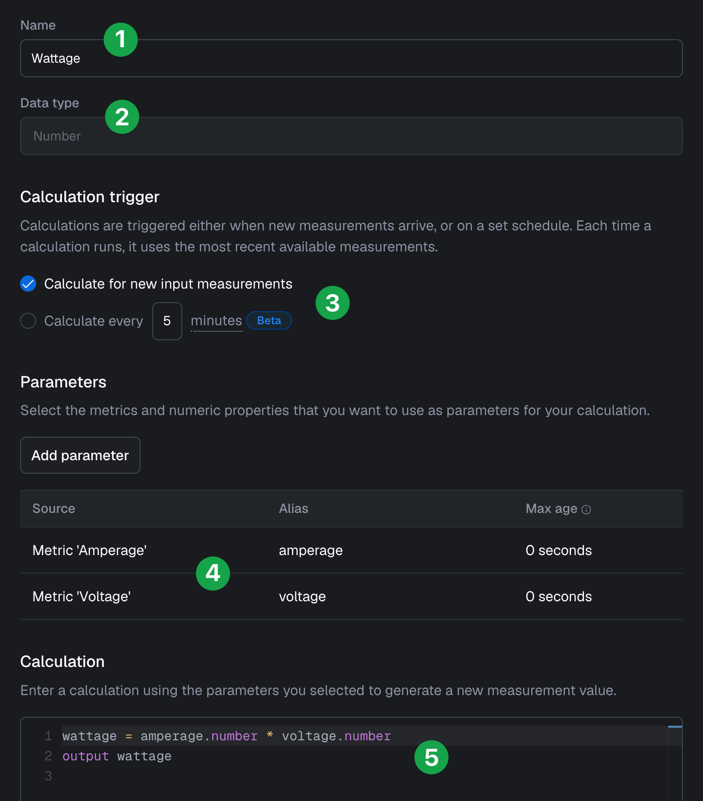
A calculated metric can be computed from the values of one or more metrics and properties within a subject. A simple example is an electrical station whose wattage is computed by multiplying voltage with amperage (shown in the examples).
The main elements of a calculation are the name (1), type (2) and trigger (3) together with the parameters (4) that can be used in the calculation (5).
Calculation trigger
A calculation can be triggered in two ways: when new measurements arrive for its input metrics, or on a set schedule.
| Trigger | Description |
|---|---|
| Calculate for new input measurements | The calculation is triggered each time a new measurement is received for one of its metric parameters. |
| Calculate every X minutes | The calculation is triggered periodically, independent of incoming measurements. Metric parameters can still be used, but are not required. |
Parameters
A calculation can use any Number, Text or Location metric or property from the subject type. These are referred to as the parameters of the calculation.
| Attribute | Description |
|---|---|
| Source | Either a metric or a property present on the subject type |
| Alias | A name without spaces that can be used to refer to the parameter in the computation |
| Max age | For metric parameters, you can set a max age, to avoid calculations on incomplete data. If a metric’s latest measurement is older than this limit, the calculation is skipped. The age is measured relative to the most recent measurement across all input metrics. |
For metrics used as parameters, you can reference both their value and date in the computation. For example, if we add a Wattage metric as parameter with alias wattage, we can use its value with wattage.number and its date in milliseconds with wattage.date.
For properties used as parameters, you can reference their value. For example, if we add a property Height with alias height, we can use its value with height.number.
The field name for the value of the metric or property differs per type:
- Numeric metrics and properties:
.number - Textual metrics and properties:
.text - Location metrics and properties:
.latitude,.longitudeand.altitude
The value of numeric and textual metrics and properties can also be retrieved with .value, but this is deprecated in favor of .number and .text.
Max age explained
To avoid calculations on incomplete data, you can set a max age. If a metric’s latest measurement is older than this limit, the calculation is skipped. The age is measured relative to the most recent measurement across all input metrics.
| Max age metric 1 | Max age metric 2 | Results |
|---|---|---|
| 0 seconds | 0 seconds | The calculation will only proceed when both metrics have a measurement with the same timestamp (in milliseconds) |
| 0 seconds | empty | Measurement for metric 1 received, the last known measurement of metric 2 will be used for the calculation. Measurement for metric 2 received, the calculation will only proceed when there is a measurement of metric 1 with the same timestamp (in milliseconds) |
| empty | 60 seconds | Measurement for metric 1 received, the calculation will proceed when there is measurement of metric 2 which is not older than 60 seconds. Measurement for metric 2 received, the last known measurement of metric 1 will be used for the calculation |
Calculation
The calculation is defined using the editor in a user-friendly language. The language allows you to:
- define variables;
- apply basic arithmetic operations;
- use functions for more advanced operations;
- save and load values in between consecutive calculations;
- use conditionals;
- output the result of your calculation.
Formulating a calculation becomes easier once you get familiar with the editor features and browse the examples.
Define variables
For readability, you can split a calculation into smaller parts and assign each part to a variable. An example of this is wattage = voltage.number * amperage.number in the example at the start of this section. This allows referring to the result of the computation voltage.number * amperage.number via the name wattage.
Arithmetic operations
All basic arithmetic operations can be applied to values in your calculation:
| Operation | Symbol | Example | Comment |
|---|---|---|---|
| Addition | + | 5 + 7 | - |
| Subtraction | - | 10 - 5 | - |
| Multiplication | * | 3 * 9 | - |
| Division | / | 10 / 2 | Division by 0 will produce no result |
| Parenthesis | ( ) | (5 + 7) * 8 | Here 5 + 7 takes precedence over multiplication by 8 |
Multiplication and division take precedence over addition and subtraction, as per the standard arithmetic rules. Any (decimal) number values, variable definitions, loaded values or input parameter values can be used in arithmetic. Operations can also be chained. Some examples:
load sum with default 0
a = voltage.number * 5.5
b = a - 7 + 8 / 2
c = sum + b
save c as sum
d = (c + 10) * 5
output d
Functions
Many default computations are available as functions. Functions can be used anywhere in your computation where a numeric value is expected, and can take as input any literal value, input parameter value, loaded value or arithmetic. For example: compute and output the maximum value of a metric parameter, with alias inputMetric, by using the max function:
load maxValue
newMaxValue = max(maxValue, inputMetric.number)
save newMaxValue as maxValue
output newMaxValue
abs(value)
Computes the absolute value of a number value.
| Parameter | Description |
|---|---|
| value | Input value to compute absolute value for |
acos(value)
Computes the angle in degrees whose cosine is the specified number.
| Parameter | Description |
|---|---|
| value | Value representing a cosine |
asin(value)
Computes the angle in degrees whose sine is the specified number.
| Parameter | Description |
|---|---|
| value | Value representing a sine |
atan(value)
Computes the angle in degrees whose tangent is the specified number.
| Parameter | Description |
|---|---|
| value | Value representing a tangent |
atan2(y,x)
Computes the angle in degrees whose tangent is the quotient of two specified numbers
| Parameter | Description |
|---|---|
| y | The y coordinate of a point |
| x | The x coordinate of a point |
ceil(value)
Rounds decimal numbers up to the closest integer value.
| Parameter | Description |
|---|---|
| value | Value to round |
cos(degrees)
Computes the cosine of the provided number of degrees.
| Parameter | Description |
|---|---|
| degrees | Input in degrees |
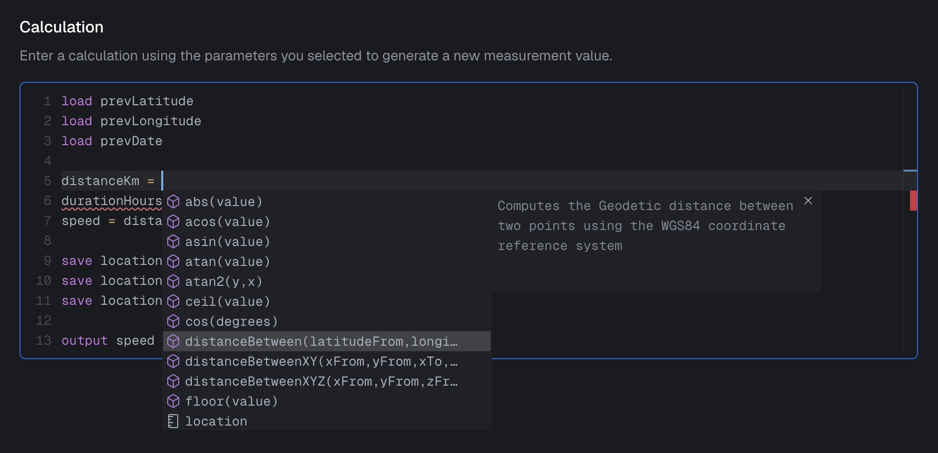
distanceBetween(latitudeFrom,longitudeFrom,latitudeTo,longitudeTo)
Computes the Geodetic (across the Earth’s surface) distance in meters between two points using the WGS84 coordinate reference system.
| Parameter | Description |
|---|---|
| latitudeFrom | From position latitude in degrees |
| longitudeFrom | From position longitude in degrees |
| latitudeTo | To position latitude in degrees |
| longitudeTo | To position latitude in degrees |
distanceBetweenXY(xFrom,yFrom,xTo,yTo)
Computes the Euclidean (straight) distance between two 2D points. Distance is in the same unit as provided coordinates.
| Parameter | Description |
|---|---|
| xFrom | From position x coordinate |
| yFrom | From position y coordinate |
| xTo | To position x coordinate |
| yTo | To position y coordinate |
distanceBetweenXYZ(xFrom,yFrom,zFrom,xTo,yTo,zTo)
Computes the Euclidean (straight) distance between two 3D points. Distance is in the same unit as provided coordinates.
| Parameter | Description |
|---|---|
| xFrom | From position x coordinate |
| yFrom | From position y coordinate |
| zFrom | From position z coordinate |
| xTo | To position x coordinate |
| yTo | To position y coordinate |
| zTo | To position z coordinate |
floor(value)
Rounds decimal numbers down to the closest integer value.
| Parameter | Description |
|---|---|
| value | Value to round |
log(value)
Computes the natural logarithm of a value.
| Parameter | Description |
|---|---|
| value | Input value to compute logarithm for |
max(value1,value2)
Computes the maximum value of two number values.
| Parameter | Description |
|---|---|
| value1 | First value to compare |
| value2 | Second value to compare |
min(value1,value2)
Computes the minimum value of two number values.
| Parameter | Description |
|---|---|
| value1 | First value to compare |
| value2 | Second value to compare |
now()
Provides the current time in milliseconds since Unix Epoch.
pi()
Provides the value of Pi with eight decimals of precision.
pow(value,power)
Computes the power of a number value.
| Parameter | Description |
|---|---|
| value | Input value to compute the power of |
| power | The power to raise the value to; fractional and negative numbers are supported |
Example: pow(3, 2) means three to the power of two which results in 9.
random(lower,upper)
Generates a random decimal number from a continuously uniform distribution between provided upper and lower bounds.
| Parameter | Description |
|---|---|
| lower | Lower bound for random number (inclusive) |
| upper | Upper bound for random number (exclusive) |
remainder(dividend,divisor)
Computes the remainder of a division. For example, the remainder of 9 / 2.5 is 1.5. The remainder always takes the sign of the dividend.
| Parameter | Description |
|---|---|
| dividend | Dividend of the division |
| divisor | Divisor of the division |
round(value,precision)
Rounds decimal numbers to a specified number of decimals. Precision rounded down to closest integer value.
| Parameter | Description |
|---|---|
| value | Value to round |
| precision | Number of decimals to round to (max 8). Decimals precision values are rounded down to nearest integer. |
sin(degrees)
Computes the sine of the provided number of degrees.
| Parameter | Description |
|---|---|
| degrees | Input in degrees |
sqrt(value)
Computes the square root of a number value.
| Parameter | Description |
|---|---|
| value | Input value to compute square root for |
tan(degrees)
Computes the tangent of the provided number of degrees.
| Parameter | Description |
|---|---|
| degrees | Input in degrees |
toDegrees(radians)
Converts an angle from radians to degrees.
| Parameter | Description |
|---|---|
| degrees | Input angle in radians |
toRadians(degrees)
Converts an angle from degrees to radians.
| Parameter | Description |
|---|---|
| degrees | Input angle in degrees |
truncateToHour(date)
Returns a new date that represents the start of the hour of the given date. Example, for February 4th, 2025 14:42:00 this will return February 4th, 2025 14:00:00. This function respects the time zone of the project. Note that dates are represented as milliseconds since Unix Epoch.
| Parameter | Description |
|---|---|
| date | Input date |
truncateToDay(date)
Returns a new date that represents the start of the day of the given date. Example, for February 4th, 2025 14:42:00 this will return February 4th, 2025 00:00:00. This function respects the time zone of the project. Note that dates are represented as milliseconds since Unix Epoch.
| Parameter | Description |
|---|---|
| date | Input date |
truncateToWeek(date)
Returns a new date that represents the start of the week of the given date. Example, for February 4th, 2025 14:42:00 this will return February 3rd, 2025 00:00:00. This function respects the time zone of the project. Note that dates are represented as milliseconds since Unix Epoch.
| Parameter | Description |
|---|---|
| date | Input date |
truncateToMonth(date)
Returns a new date that represents the start of the month of the given date. Example, for February 4th, 2025 14:42:00 this will return February 1st, 2025 00:00:00. This function respects the time zone of the project. Note that dates are represented as milliseconds since Unix Epoch.
| Parameter | Description |
|---|---|
| date | Input date |
Save and load values
It is possible to save and load values between consecutive evaluations of the calculation. A numeric value can be saved at the end of a calculation, so that it can be loaded the next time the calculation is evaluated. A maximum of 10 values can be saved and if a value exceeds 8 decimal places, it will be rounded off. For example: we want to compare the value of a metric to its previous value.
load previousValue
difference = bitcoin.number - previousValue
save bitcoin.number as previousValue
output difference
Values must be loaded at the beginning of a calculation with a name that is later used to save the value. See load previousValue will create a variable with name previousValue. If a variable is loaded, a value must be saved in it at some point during the calculation. See save bitcoin.number as previousValue which saves the current bitcoin metric value in previousValue to be used by the next evaluation of the calculation.
It is possible to use the value of a loaded variable to update its own value. For example when we are keeping a sum:
load bitcoinSum with default 0
newSum = bitcoinSum + bitcoin.number
save newSum as bitcoinSum
output newSum
In this case a default must be provided when loading the variable, see load valueSum with default 0. The default is used on the first evaluation, before any value has been saved. Without it, the variable could never be initialized.
Conditionals
The editor supports conditionals so you can vary the calculation based on the input values. Use if, then and else statements, and combine conditions with and or or.
if-then-else
If-then-else statements are used to allow conditional execution of statements. A condition needs to be stated after the if statement. If the said condition is true, the then value will be used. If the condition returns false the else value will be used.
if <condition> then <value1> else <value2>
checking for equality
A condition can check whether two values are the same or not with the operators == (equal to) and != (not equal to). This is supported for both numeric:
voltage.number == 230
and textual values:
soilType.text != "Peat moss"
comparing numbers
Numbers can also be compared with the operators > (greater than), >= (greater than or equal to), < (less than), and <= (less than or equal to):
temperature.number > 25
and
The and operator combines two conditions; it returns true only when both conditions are true. If either condition is false, the operator returns false.
The syntax can be seen below:
<condition1> and <condition2>
To illustrate how you can combine if, then and else statements with and, see the sample syntax below:
if <condition1> and <condition2> then <value1> else <value2>
or
The or operator combines two conditions; it returns true when at least one of them is true.
<condition1> or <condition2>
To illustrate how you can combine if, then and else statements with or, see the sample syntax below:
if <condition1> or <condition2> then <value1> else <value2>
hasValue
With a hasValue condition, you can check whether a metric or property has a value. By default, referencing a metric with no measurement terminates the calculation and produces no output. Use hasValue when you want to branch on the presence of a value instead:
setpoint = if hasValue(setpointManual.number)
           then setpointManual.number
           else setpointSchedule.number
Output
Each calculation must specify exactly one output value at the end of the calculation as follows: output <value>. In this case <value> can be any (decimal) number value, arithmetic, variable definition, loaded value or parameter value.
- A calculated metric is triggered as configured; when a measurement for one of its parameters arrives, or on a schedule.
- A calculation will only take place when all variables within the calculation are present.
- Above condition holds for each saved value and output independently. So a loaded value could be saved in a previous evaluation while no output was generated.
- If an output value exceeds 8 decimal places, it will be rounded off.
Editor features
The editor has a few features that aren’t immediately visible but make it much easier to use. They’re listed in the table below.
| Feature | Action | Description |
|---|---|---|
| Extra info | hover | Use the mouse to hover over the elements in the editor to see extra information. |
| Option list | ctrl + space | Get to see the list options you can select in the current context. |
| Option description | ctrl + space | Hit ctrl + space a second time to see the description of the option. |
| Commenting | // or /* ... */ | Put // at the start of a line to write a single-line comment. Alternatively start a multi-line comment with /* and end it with */ |
| Red underline | N/A | A (part of) the calculation has a red underline when the editor detects a possible mistake. Hover the red underline for more details and suggestions. |
Examples
This section walks through a few examples to make calculated metrics concrete and illustrate the settings.
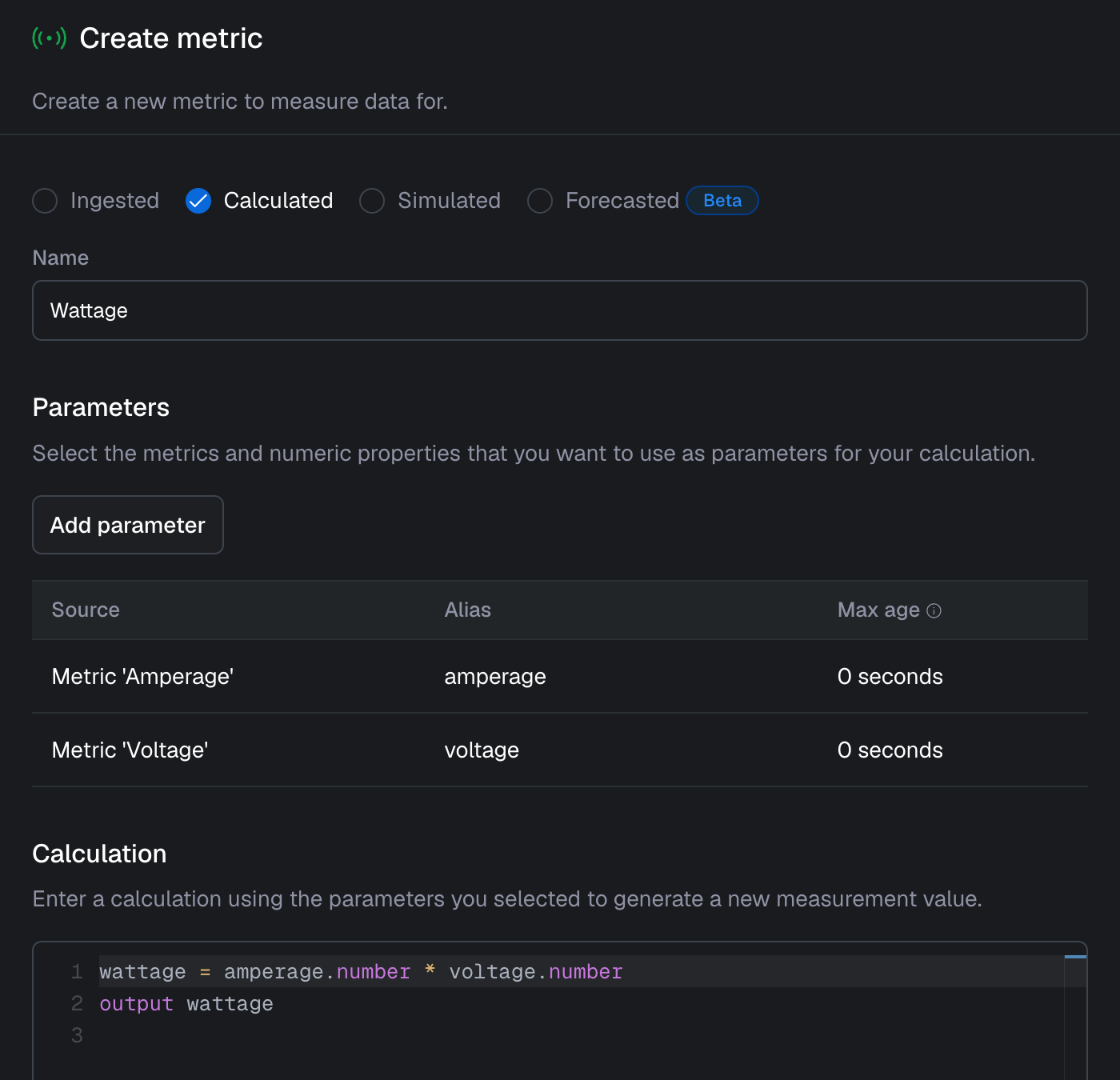
Wattage calculation
The wattage will only be calculated when voltage and amperage are received with the same timestamp. This is because both parameters have a max age of zero seconds.
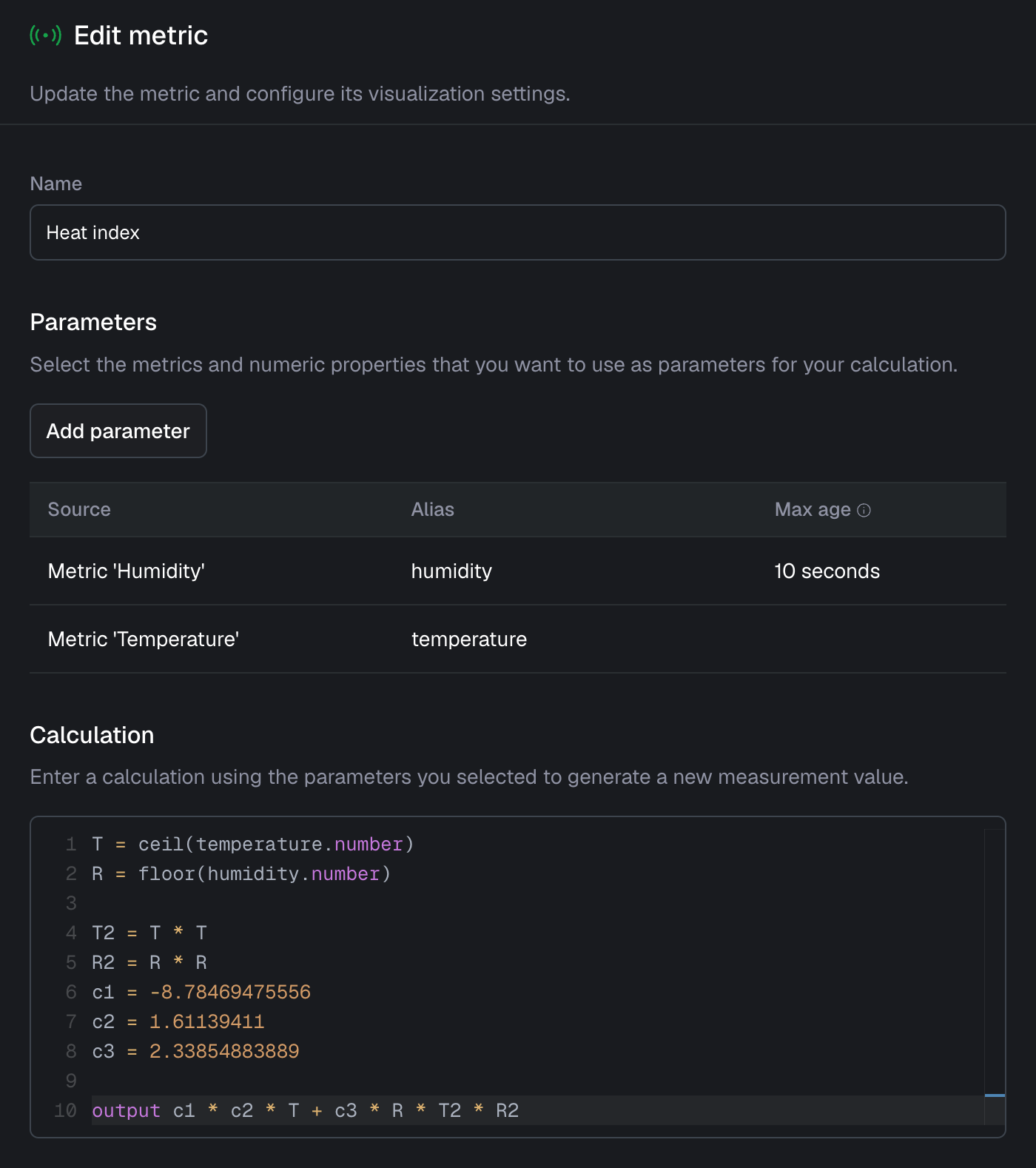
Heat index
The heat index will be calculated with the last known temperature measurement when the humidity measurement is received and with a humidity measurement not older than 10 seconds when a temperature measurement is received.
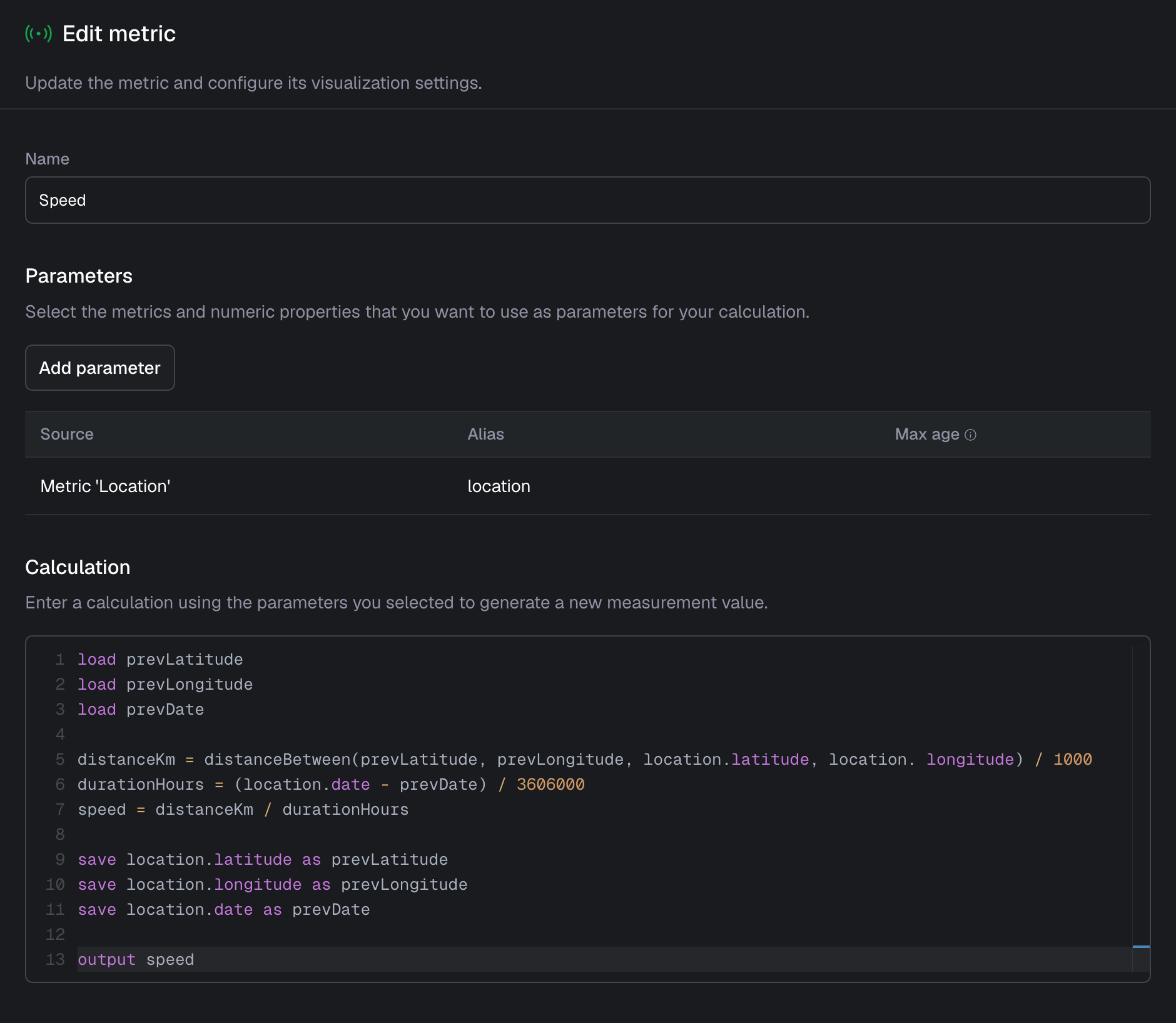
Speed
The speed is calculated with the last known location which contains the latitude, longitude and date values. This example includes save and load values, functions and arithmetic operations which all together shows the power and possibilities of a calculated metric.
Load Factor
In order to calculate the load factor, there are various conditions that need to be met in order to create a representative calculated metric. In this case, we are calculating the load factor when rP and qP are both positive, else a 0 value is returned as output for the calculated metric. This example shows the ability to use conditionals.
Aggregations over specific periods
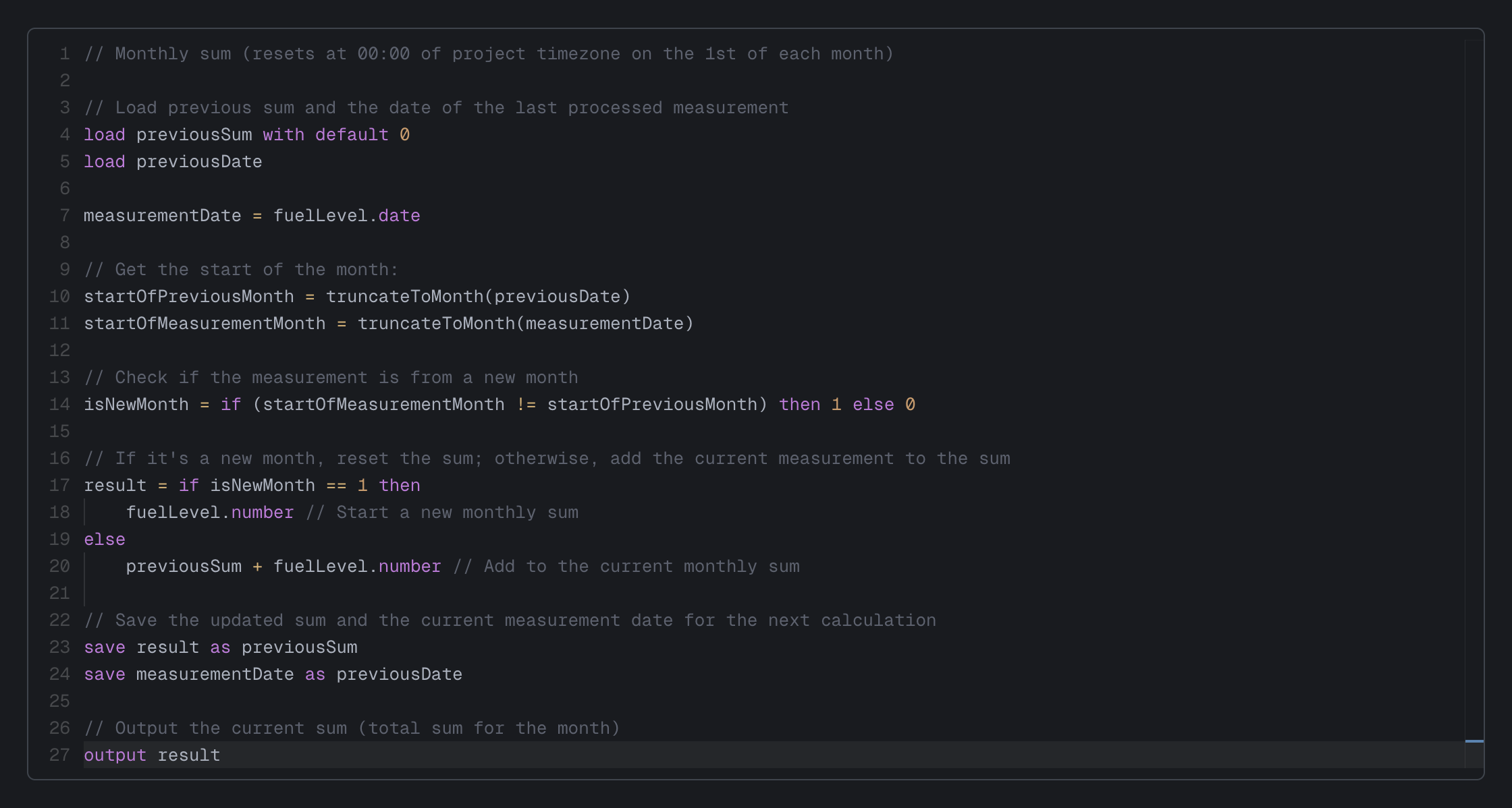
Aggregations can be used when you want to keep track of for example your monthly fuel usage. Using the date function truncateTo[Hour|Day|Week|Month] it is possible to make various aggregations per hour, day, week or month which results can be used in triggers, graphs, tables and other visualizations. This is an example for your monthly fuel usage:
Simulated metric
A simulated metric generates data based on the configuration. Example: a two hour sinus.
| Attribute | Description |
|---|---|
| Name | Give the simulated metric a descriptive name so you can easily recognize and find it. |
| Simulation type | Choose between a random walk and sinus two hours. |
| Measurement interval | Choose with which frequency measurements are generated. |
| Value lower bound | Determine what the lowest value will be for the measurements that are generated. |
| Value upper bound | Determine what the highest value will be for the measurements that are generated. |
Forecasted metric
A forecasted metric allows you to forecast future values of an existing metric. To achieve this, a model to forecast future values is created under the hood using artificial intelligence (AI), specifically deep learning. The model is created by training on historical data to learn patterns and trends. A new incoming measurement on the metric to forecast will instantly be inferred by the model, resulting in a new measurement on the forecasted metric with its forecasted future value and future date. Conceptually, it is thus quite similar to a calculated metric.
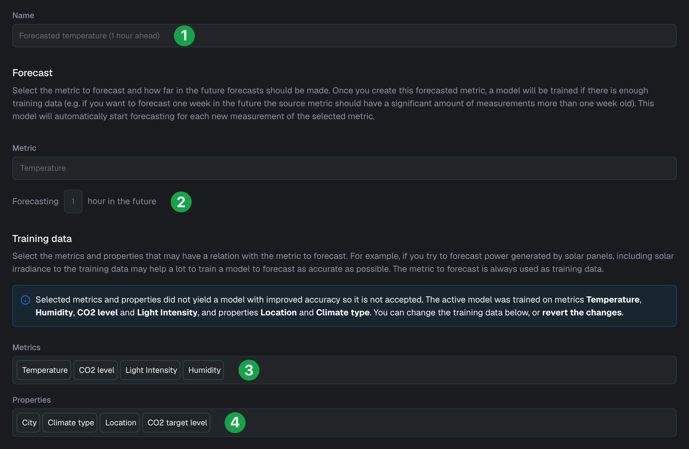
The main elements of a forecasted metric are the name (1), the metric and time in the future to forecast (2), and its training data, which can be existing metrics (3) or properties (4).
Training data
One of the key success criteria for getting accurate forecasts is the training data we use to train a model. By experimenting with different training data, you can significantly improve your model. Once you select new data and save the metric, it will immediately start training on this new data; it will only accept and use models if they result in improved forecast accuracy. The metrics you use as training data should have enough historical measurements (e.g., if you want to forecast one week in the future, the metrics should have a significant amount of measurements that are more than one week old).
To make data more useful for a model, it can be beneficial not just to add the existing metrics to the training data but also to construct new metrics to make them more useful for the model. This part of developing a model is called feature engineering, which is often overlooked while being vital to success. For example, you could use the rate of increase or decrease as a feature instead of simply the value of a metric. We could also engineer features based on the date and time, such as whether it is day or night or a working day or not. In order to achieve this, you can for instance create new calculated metrics and add them as training data.
Forecast accuracy
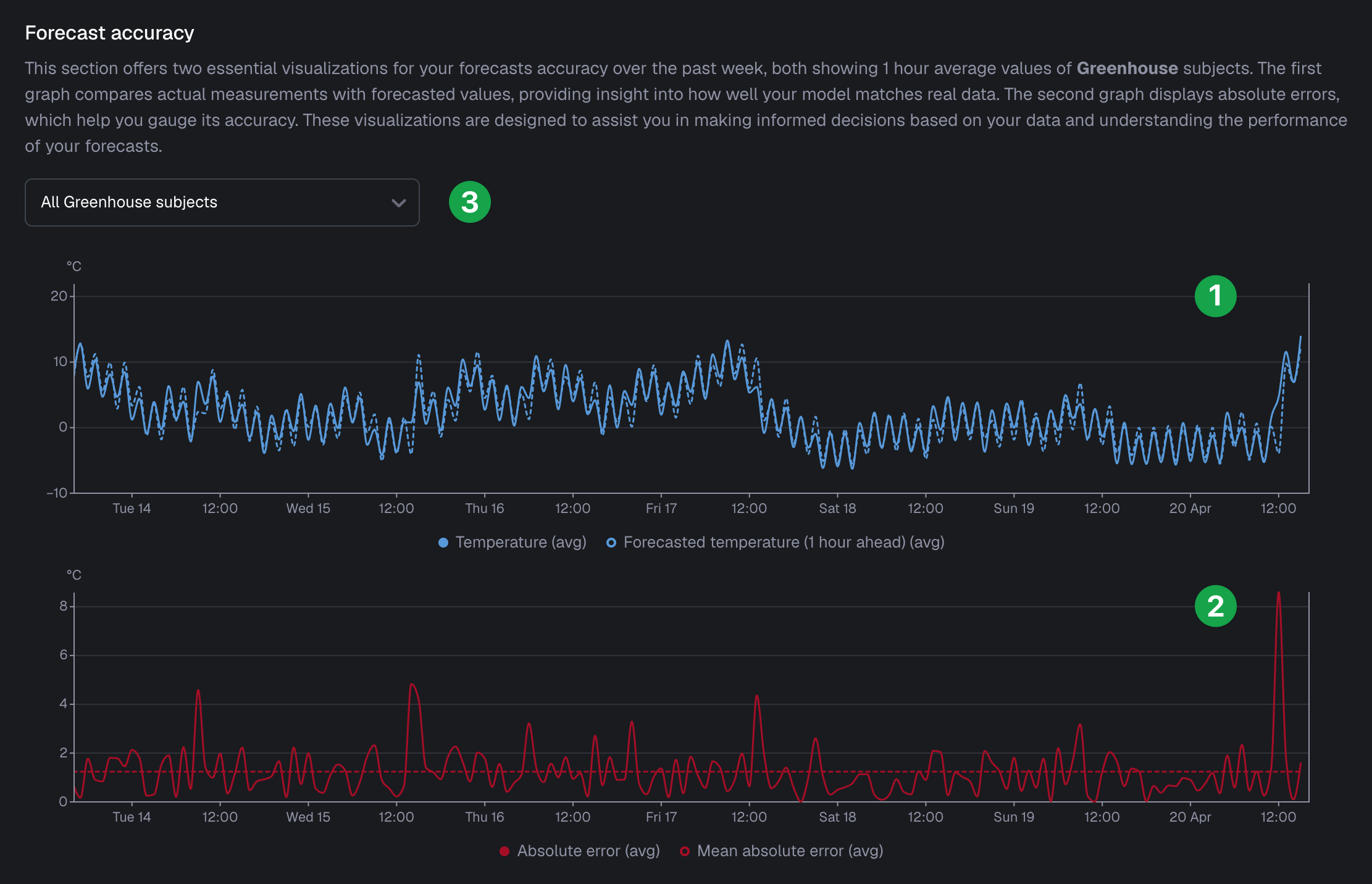
To monitor the accuracy of your forecasts, two key graphs are available for evaluating averaged hourly forecast accuracy over the past week. The first graph (1) compares actual measurements with forecasted values, providing insight into how well your forecast matches real data. The second graph (2) displays absolute errors, offering a clear indication of forecast accuracy. You can choose to view aggregated accuracy metrics for all subjects or focus on a specific subject (3).
Immediately following the initial training, these graphs are populated with forecasts from one week prior, providing an immediate assessment of the model’s performance. Note that data from this period is not used for training, ensuring that it gives a good, i.e., unbiased, indication of the expected accuracy.
Recent trainings
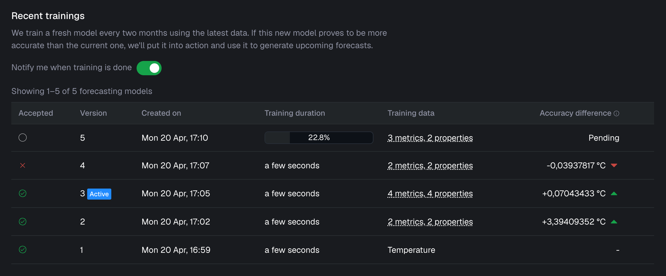
After initial training, any changes to inputs trigger a new training. By default, the platform also retrains a model automatically every two months to ensure new observations are taken into account. Models that achieve higher accuracy are accepted and used automatically, while models that are not accepted are only shown in the recent trainings overview. The accuracy difference is determined by using the active model and the newly trained model to make forecasts for test data that has not been used for training.
A green check mark indicates an accepted model, while a red cross indicates that it is not accepted. The version of the model is displayed, with active models marked by an active badge. The creation date of each model is also displayed. Training duration information includes training times for completed models and a progress bar for models currently in training. The training data contains a history of the input metrics and properties used for each training version, which users can hover over to see the composition of input metrics and properties. The accuracy comparison shows the difference in absolute error compared to the previous active model, with positive values indicating an improvement in error by that amount. Lastly, users can enable notifications for updates on training completion.
If altering the model’s inputs doesn’t improve accuracy, the changes can be easily undone.
Explore
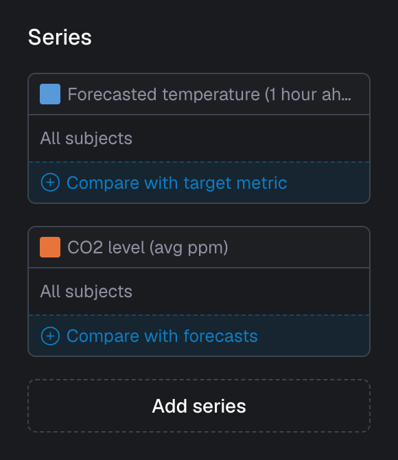
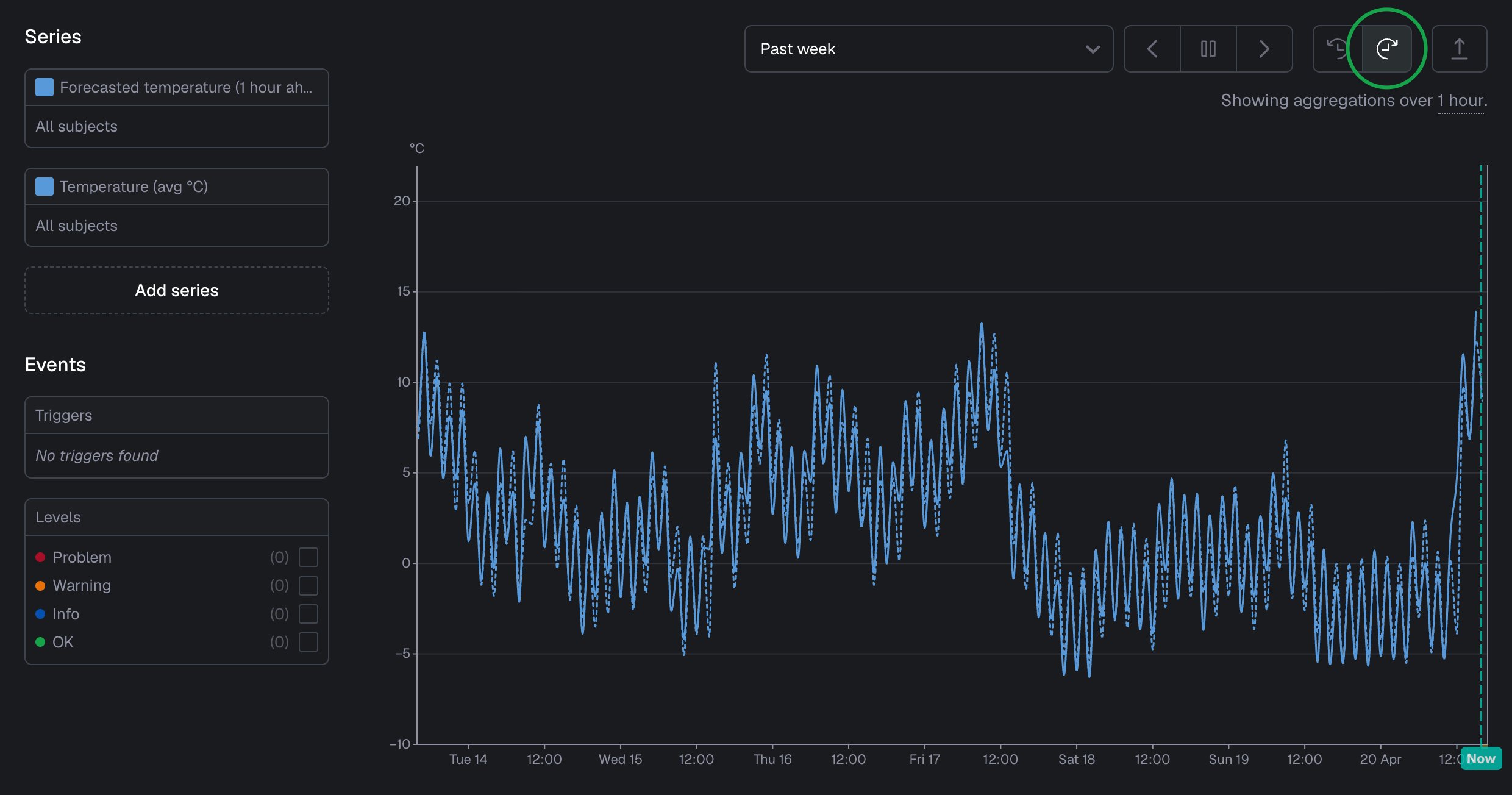
Users can use the Blockbax Explorer to analyze and compare forecasted metrics with actual observed values. When a forecasted metric is selected, the Explorer suggests comparing it with the target metric. Likewise, selecting the target metric offers a comparison with its forecasts.
Conceptually, we consider a forecast to be measured (i.e., determined) at the same time as the measurement that triggers the forecast. In the Explorer, you can thus easily match the triggering measurement with the resulting forecast. Of course, in most cases, you are more interested in aligning with the time a metric forecasts for. This is enabled by default when you select a forecasted metric in the Explorer (click the circled button in the image below to align using measurement time).
Case studies
We compiled blogs featuring case studies that can inspire your own use cases.

Forecasting water quality using AI
October 23, 2024 · 12 min read
Important to keep in mind:
- It is highly use case dependent if historic data can be accurately forecasted. Some use cases are inherently hard, or might even be impossible, to forecast.
- Forecasted metrics use machine learning technology, which can sometimes result in inaccurate, inappropriate, or biased outcomes. Decisions based on machine learning outputs, including those used for automation, should have human oversight and review processes to ensure forecasts are accurate.
- From time to time, we may refine the forecasting algorithm. Such improvements roll out through the regular release process. While you cannot revert to a previous version of the feature, models already created and still active will continue using the same version.
